Support Vector Data Description (SVDD)

Python code for abnormal detection or fault detection using Support Vector Data Description (SVDD)

Version 1.1, 11-NOV-2021

Email: iqiukp@outlook.com

Main features

• SVDD BaseEstimator based on sklearn.base for one-class or binary classification
• Multiple kinds of kernel functions (linear, gaussian, polynomial, sigmoid)
• Visualization of decision boundaries for 2D data

Requirements

• cvxopt
• matplotlib
• numpy
• scikit_learn
• scikit-opt (optional, only used for parameter optimization)

Notices

• The label must be 1 for positive sample or -1 for negative sample.
• Detailed applications please see the examples.
• This code is for reference only.

Examples

01. svdd_example_unlabeled_data.py

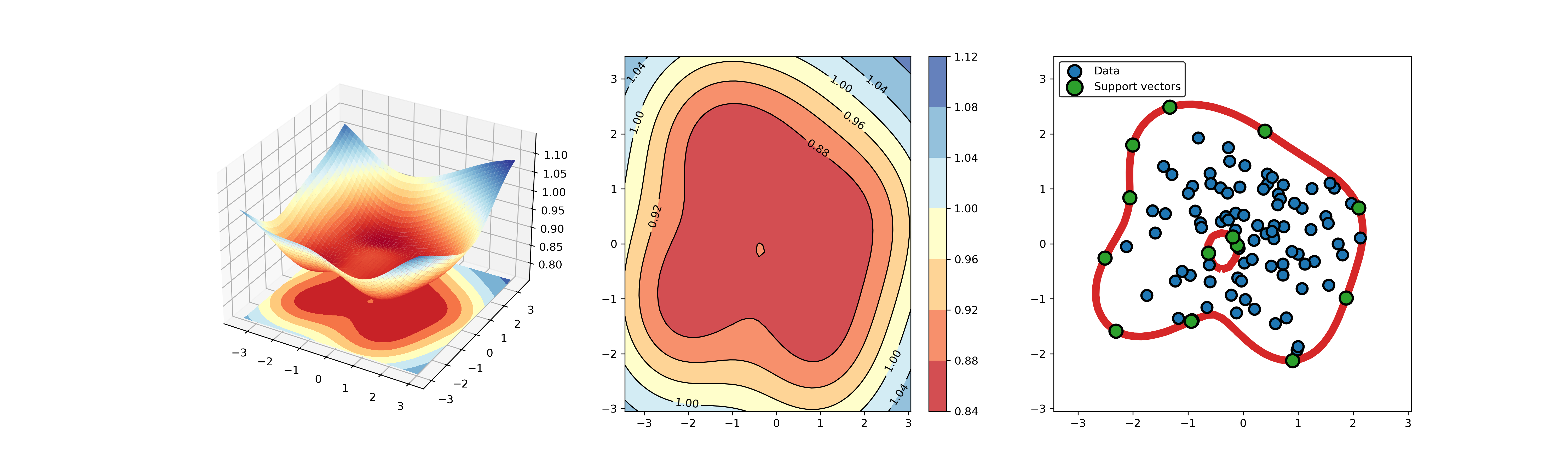
An example for SVDD model fitting using unlabeled data.

02. svdd_example_hybrid_data.py

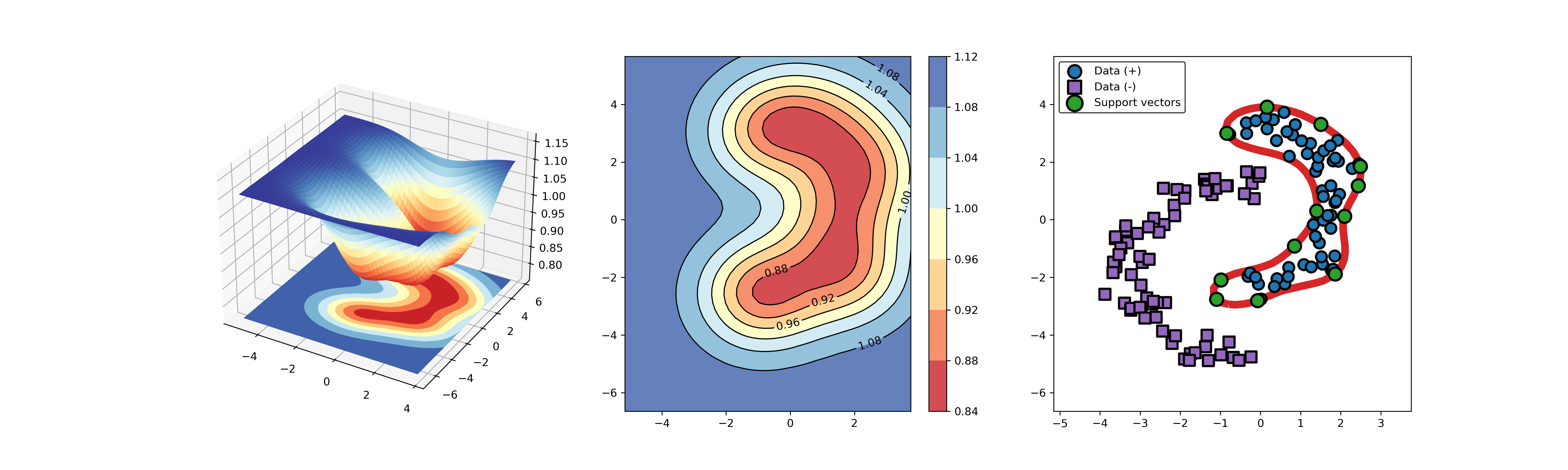
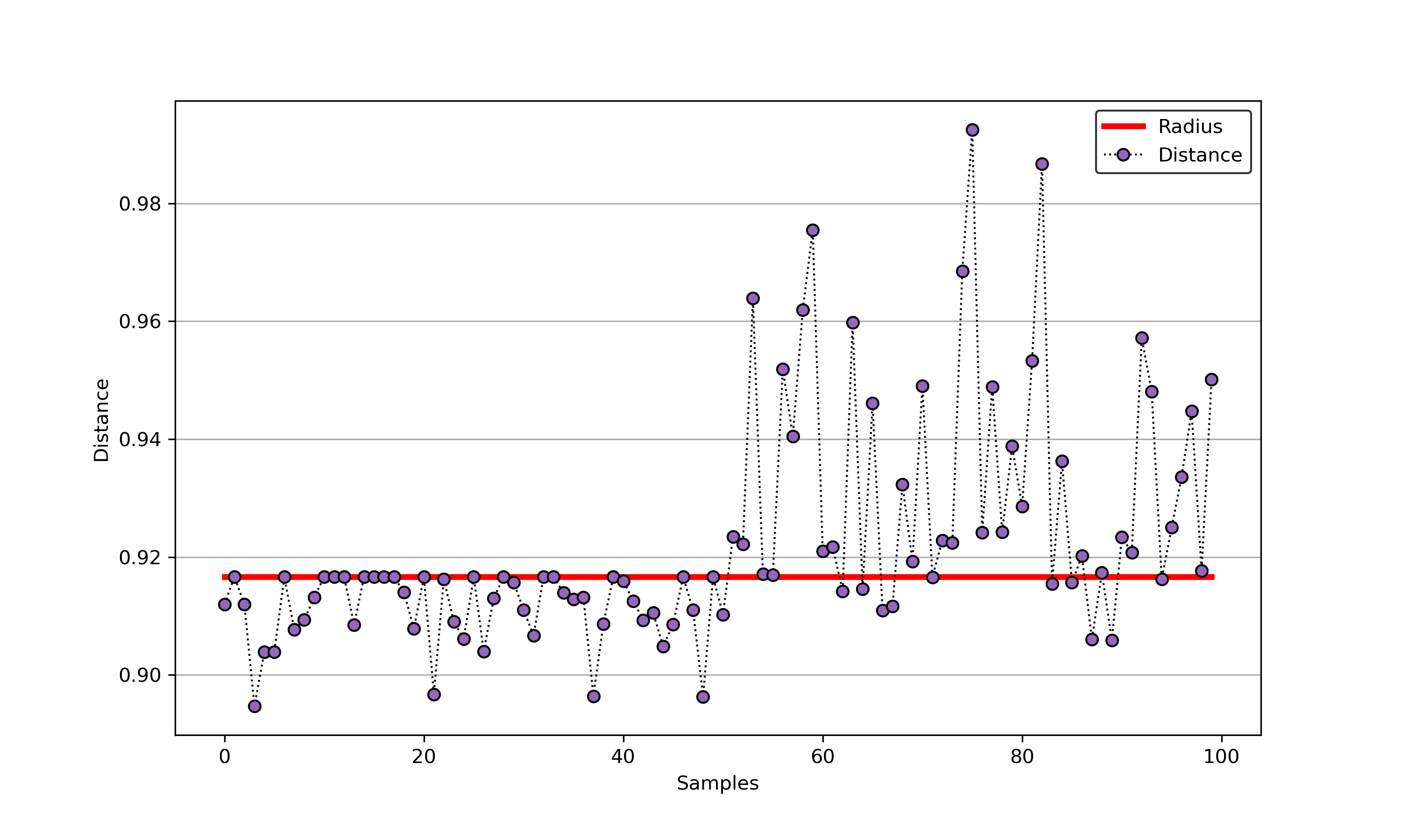
An example for SVDD model fitting with negataive samples.

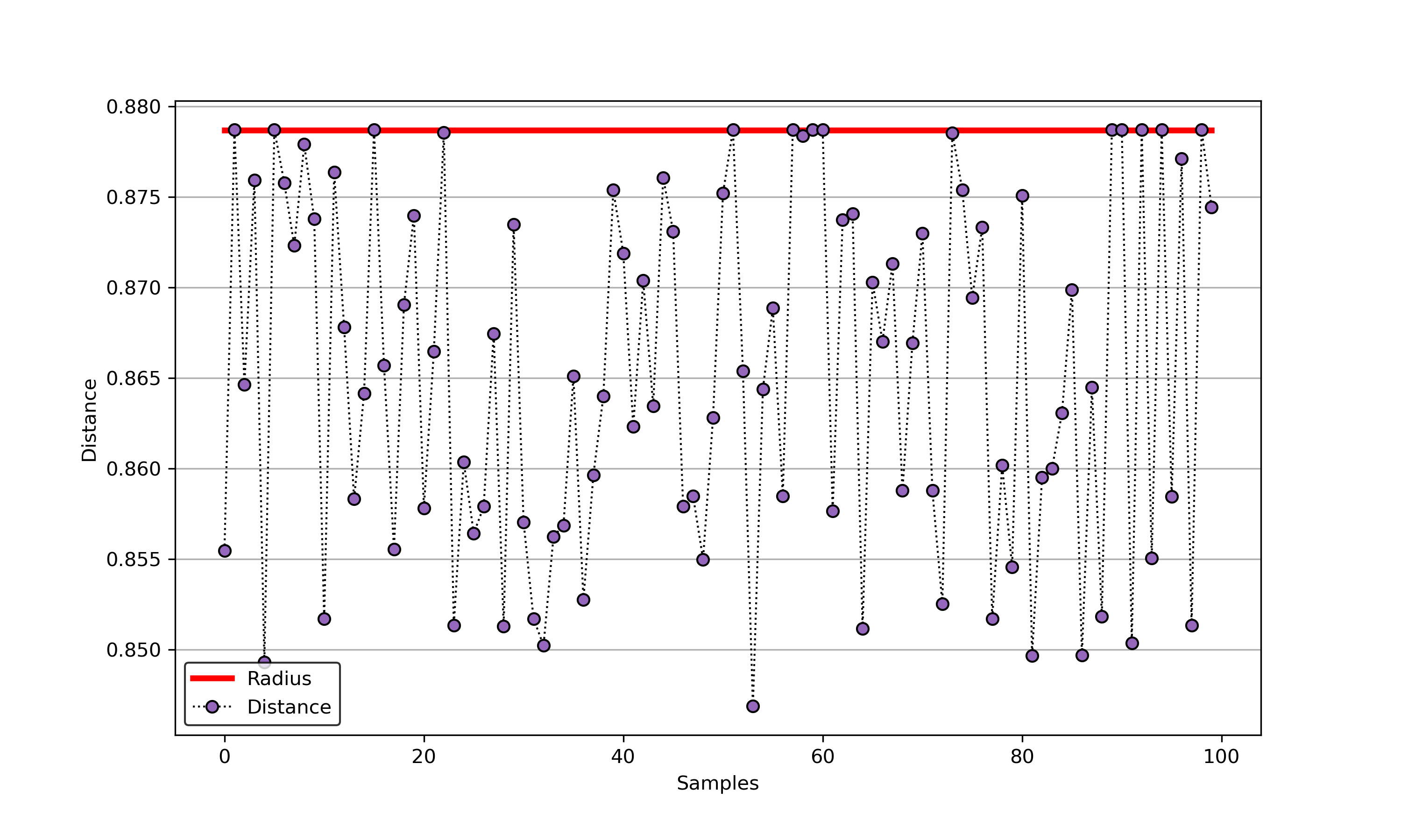
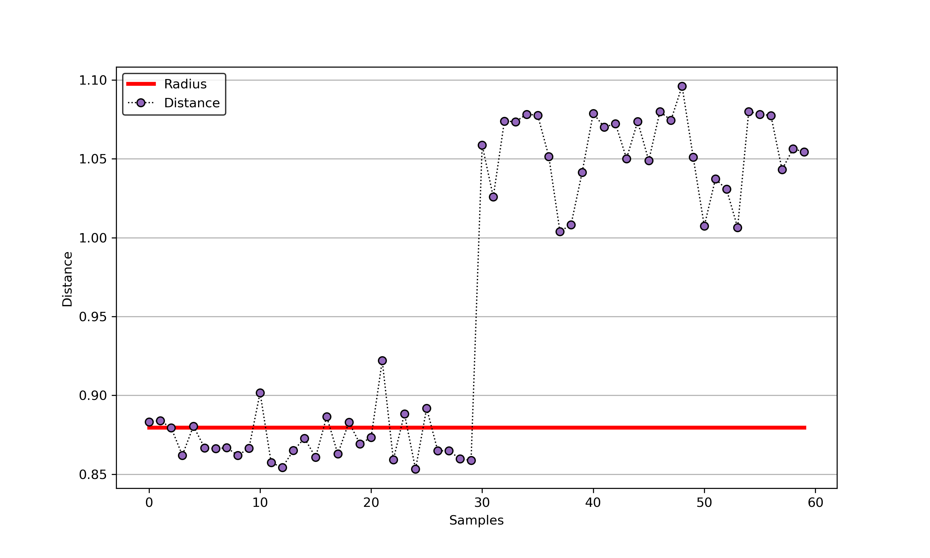
import sys
sys.path.append("..")
from sklearn.datasets import load_wine
from src.BaseSVDD import BaseSVDD, BananaDataset
# Banana-shaped dataset generation and partitioning
X, y = BananaDataset.generate(number=100, display='on')
X_train, X_test, y_train, y_test = BananaDataset.split(X, y, ratio=0.3)
# 
svdd = BaseSVDD(C=0.9, gamma=0.3, kernel='rbf', display='on')
# 
svdd.fit(X_train,  y_train)
# 
svdd.plot_boundary(X_train,  y_train)
#
y_test_predict = svdd.predict(X_test, y_test)
#
radius = svdd.radius
distance = svdd.get_distance(X_test)
svdd.plot_distance(radius, distance)

03. svdd_example_kernel.py

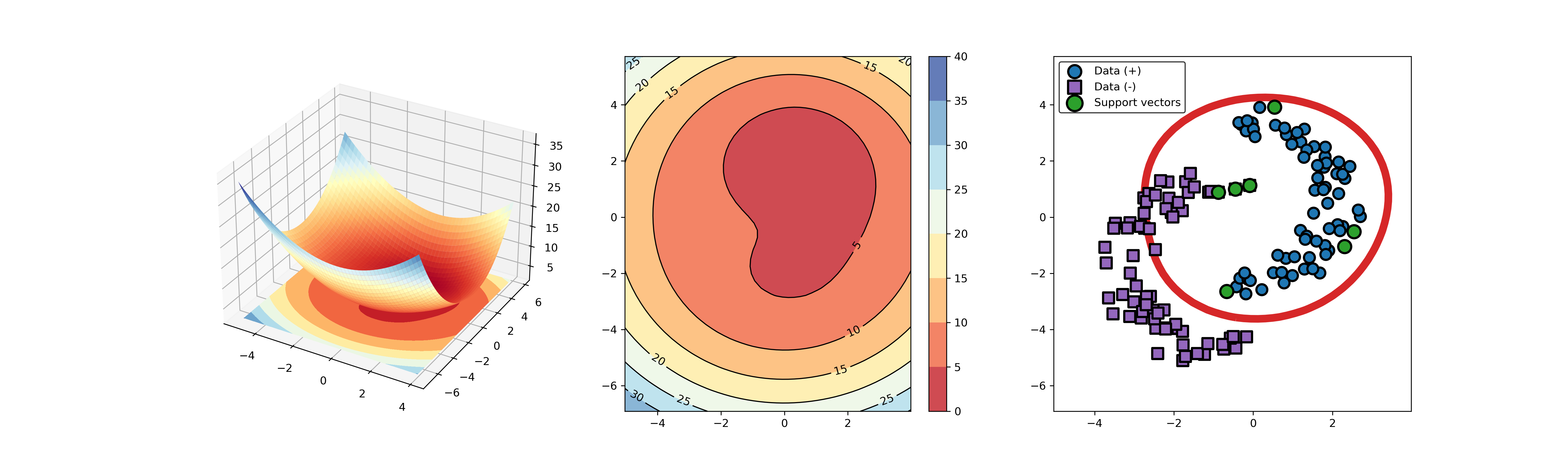
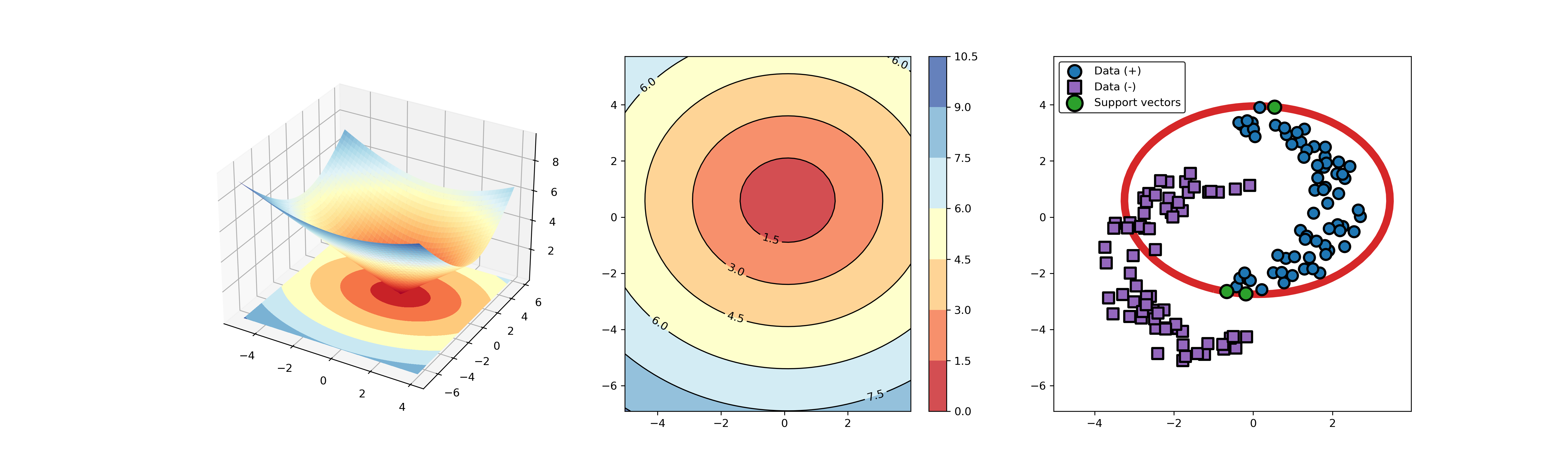
An example for SVDD model fitting using different kernels.

import sys
sys.path.append("..")
from src.BaseSVDD import BaseSVDD, BananaDataset
# Banana-shaped dataset generation and partitioning
X, y = BananaDataset.generate(number=100, display='on')
X_train, X_test, y_train, y_test = BananaDataset.split(X, y, ratio=0.3)
# kernel list
kernelList = {"1": BaseSVDD(C=0.9, kernel='rbf', gamma=0.3, display='on'),
              "2": BaseSVDD(C=0.9, kernel='poly',degree=2, display='on'),
              "3": BaseSVDD(C=0.9, kernel='linear', display='on')
              }
# 
for i in range(len(kernelList)):
    svdd = kernelList.get(str(i+1))
    svdd.fit(X_train,  y_train)
    svdd.plot_boundary(X_train,  y_train)

04. svdd_example_KPCA.py

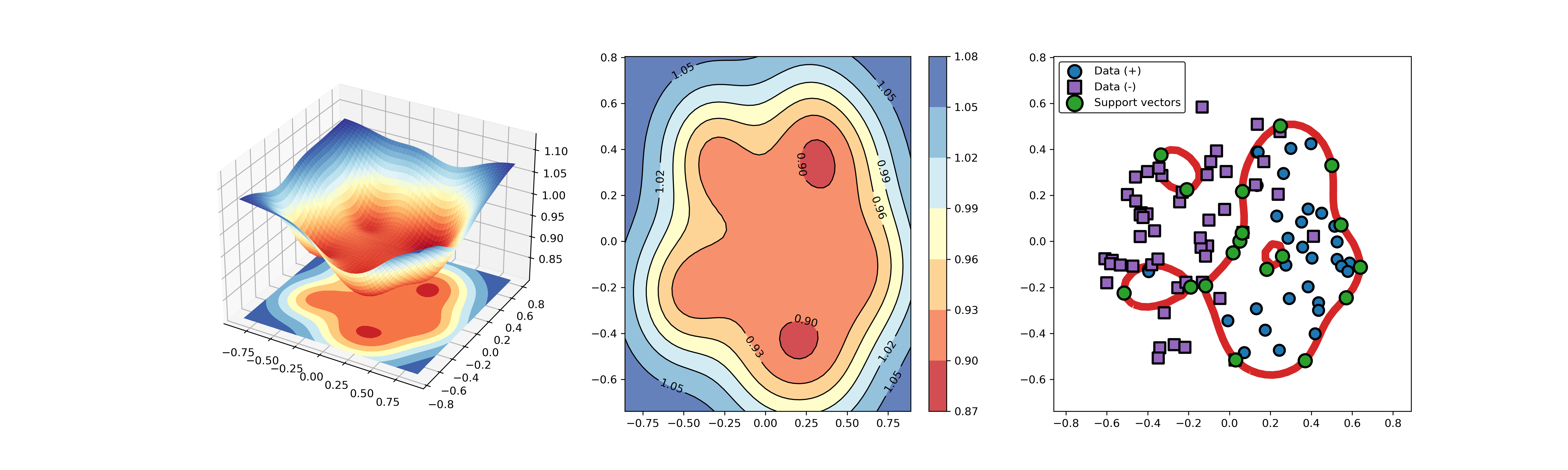
An example for SVDD model fitting using nonlinear principal component.

The KPCA algorithm is used to reduce the dimension of the original data.

import sys
sys.path.append("..")
import numpy as np
from src.BaseSVDD import BaseSVDD
from sklearn.decomposition import KernelPCA
# create 100 points with 5 dimensions
X = np.r_[np.random.randn(50, 5) + 1, np.random.randn(50, 5)]
y = np.append(np.ones((50, 1), dtype=np.int64), 
              -np.ones((50, 1), dtype=np.int64),
              axis=0)
# number of the dimensionality
kpca = KernelPCA(n_components=2, kernel="rbf", gamma=0.1, fit_inverse_transform=True)
X_kpca = kpca.fit_transform(X)
# fit the SVDD model
svdd = BaseSVDD(C=0.9, gamma=10, kernel='rbf', display='on')
# fit and predict
svdd.fit(X_kpca,  y)
y_test_predict = svdd.predict(X_kpca, y)
# plot the distance curve
radius = svdd.radius
distance = svdd.get_distance(X_kpca)
svdd.plot_distance(radius, distance)
# plot the boundary
svdd.plot_boundary(X_kpca,  y)

05. svdd_example_PSO.py

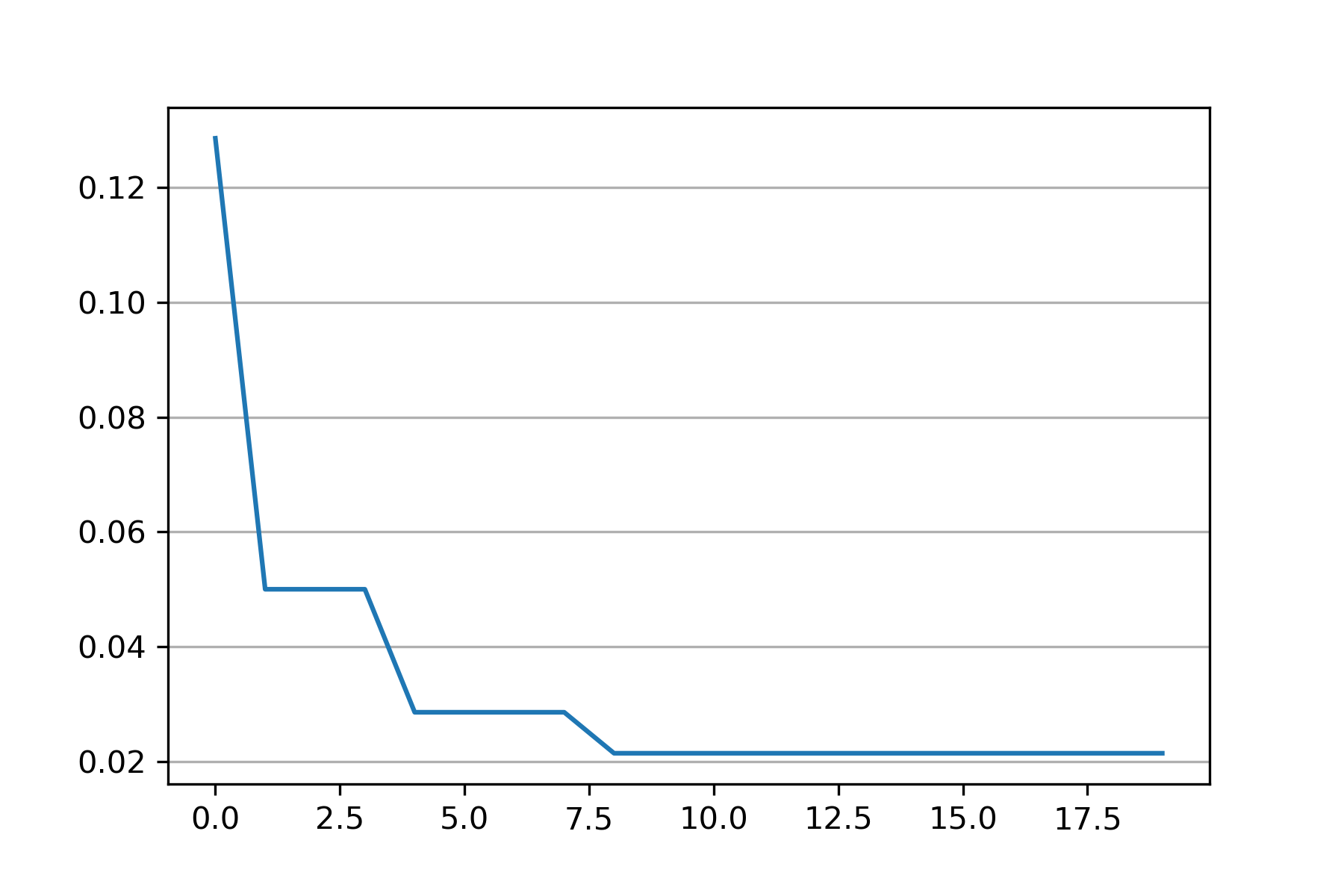
An example for parameter optimization using PSO.

“scikit-opt” is required in this example.

https://github.com/guofei9987/scikit-opt

import sys
sys.path.append("..")
from src.BaseSVDD import BaseSVDD, BananaDataset
from sko.PSO import PSO
import matplotlib.pyplot as plt
# Banana-shaped dataset generation and partitioning
X, y = BananaDataset.generate(number=100, display='off')
X_train, X_test, y_train, y_test = BananaDataset.split(X, y, ratio=0.3)
# objective function
def objective_func(x):
    x1, x2 = x
    svdd = BaseSVDD(C=x1, gamma=x2, kernel='rbf', display='off')
    y = 1-svdd.fit(X_train, y_train).accuracy
    return y
# Do PSO
pso = PSO(func=objective_func, n_dim=2, pop=10, max_iter=20, 
          lb=[0.01, 0.01], ub=[1, 3], w=0.8, c1=0.5, c2=0.5)
pso.run()
print('best_x is', pso.gbest_x)
print('best_y is', pso.gbest_y)
# plot the result
fig = plt.figure(figsize=(6, 4))
ax = fig.add_subplot(1, 1, 1)
ax.plot(pso.gbest_y_hist)
ax.yaxis.grid()
plt.show()

06. svdd_example_confusion_matrix.py

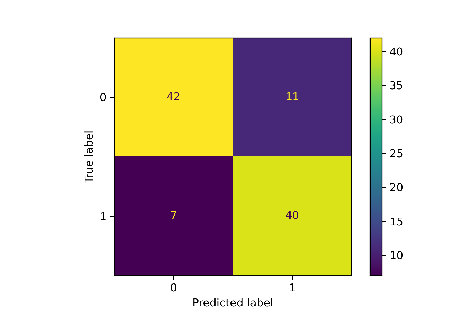
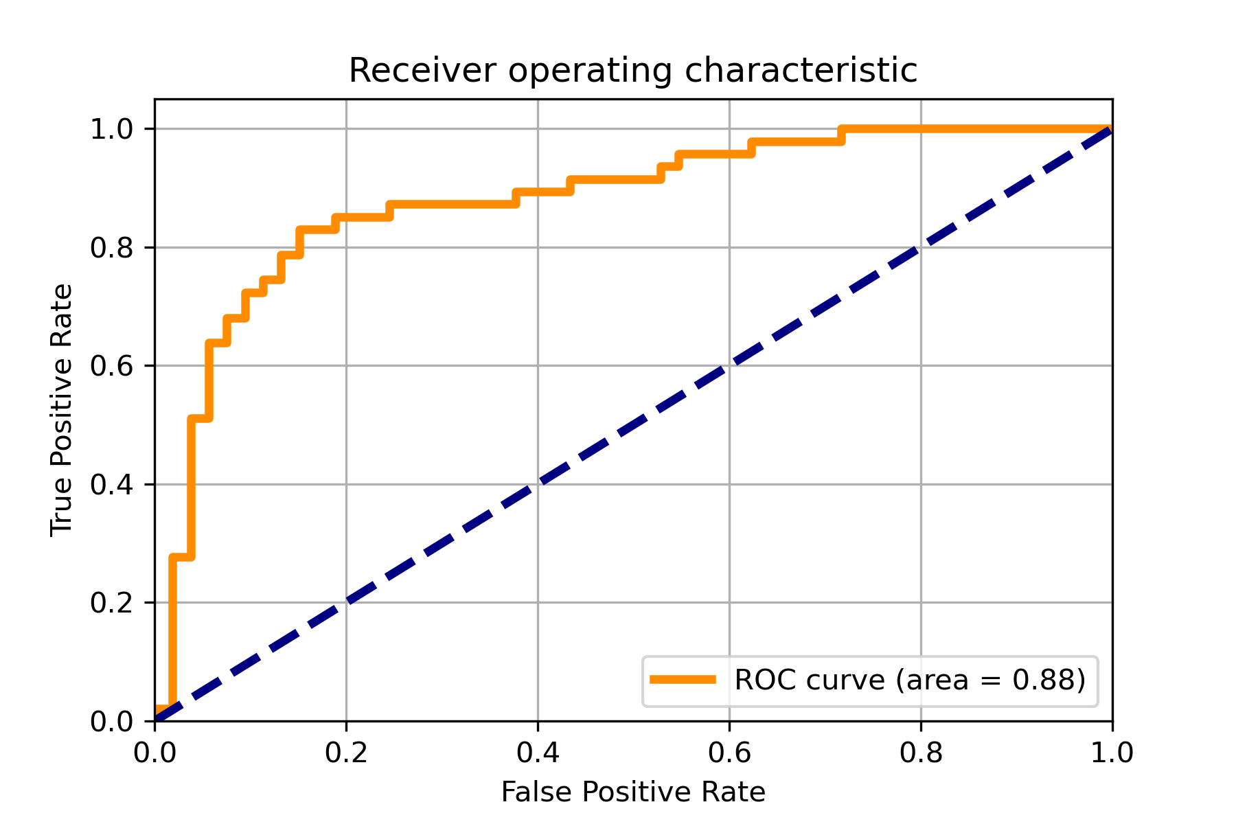
An example for drawing the confusion matrix and ROC curve.

07. svdd_example_cross_validation.py

An example for cross validation.

import sys
sys.path.append("..")
from src.BaseSVDD import BaseSVDD, BananaDataset
from sklearn.model_selection import cross_val_score
# Banana-shaped dataset generation and partitioning
X, y = BananaDataset.generate(number=100, display='on')
X_train, X_test, y_train, y_test = BananaDataset.split(X, y, ratio=0.3)
# 
svdd = BaseSVDD(C=0.9, gamma=0.3, kernel='rbf', display='on')
# cross validation (k-fold)
k = 5
scores = cross_val_score(svdd, X_train, y_train, cv=k, scoring='accuracy')
#
print("Cross validation scores:")
for scores_ in scores:
    print(scores_)
print("Mean cross validation score: {:4f}".format(scores.mean()))

Results

Cross validation scores:
0.5714285714285714
0.75
0.9642857142857143
1.0
1.0
Mean cross validation score: 0.857143

08. svdd_example_grid_search.py

An example for parameter selection using grid search.

import sys
sys.path.append("..")
from sklearn.datasets import load_wine
from src.BaseSVDD import BaseSVDD, BananaDataset
from sklearn.model_selection import KFold, LeaveOneOut, ShuffleSplit
from sklearn.model_selection import learning_curve, GridSearchCV
# Banana-shaped dataset generation and partitioning
X, y = BananaDataset.generate(number=100, display='off')
X_train, X_test, y_train, y_test = BananaDataset.split(X, y, ratio=0.3)
param_grid = [
    {"kernel": ["rbf"], "gamma": [0.1, 0.2, 0.5], "C": [0.1, 0.5, 1]},
    {"kernel": ["linear"], "C": [0.1, 0.5, 1]},
    {"kernel": ["poly"], "C": [0.1, 0.5, 1], "degree": [2, 3, 4, 5]},
]
svdd = GridSearchCV(BaseSVDD(display='off'), param_grid, cv=5, scoring="accuracy")
svdd.fit(X_train, y_train)
print("best parameters:")
print(svdd.best_params_)
print("\n")
# 
best_model = svdd.best_estimator_
means = svdd.cv_results_["mean_test_score"]
stds = svdd.cv_results_["std_test_score"]
for mean, std, params in zip(means, stds, svdd.cv_results_["params"]):
    print("%0.3f (+/-%0.03f) for %r" % (mean, std * 2, params))
print()

Results

best parameters:
{'C': 0.5, 'gamma': 0.1, 'kernel': 'rbf'}
0.921 (+/-0.159) for {'C': 0.1, 'gamma': 0.1, 'kernel': 'rbf'}
0.893 (+/-0.192) for {'C': 0.1, 'gamma': 0.2, 'kernel': 'rbf'}
0.857 (+/-0.296) for {'C': 0.1, 'gamma': 0.5, 'kernel': 'rbf'}
0.950 (+/-0.086) for {'C': 0.5, 'gamma': 0.1, 'kernel': 'rbf'}
0.921 (+/-0.131) for {'C': 0.5, 'gamma': 0.2, 'kernel': 'rbf'}
0.864 (+/-0.273) for {'C': 0.5, 'gamma': 0.5, 'kernel': 'rbf'}
0.950 (+/-0.086) for {'C': 1, 'gamma': 0.1, 'kernel': 'rbf'}
0.921 (+/-0.131) for {'C': 1, 'gamma': 0.2, 'kernel': 'rbf'}
0.864 (+/-0.273) for {'C': 1, 'gamma': 0.5, 'kernel': 'rbf'}
0.807 (+/-0.246) for {'C': 0.1, 'kernel': 'linear'}
0.821 (+/-0.278) for {'C': 0.5, 'kernel': 'linear'}
0.793 (+/-0.273) for {'C': 1, 'kernel': 'linear'}
0.879 (+/-0.184) for {'C': 0.1, 'degree': 2, 'kernel': 'poly'}
0.836 (+/-0.305) for {'C': 0.1, 'degree': 3, 'kernel': 'poly'}
0.771 (+/-0.416) for {'C': 0.1, 'degree': 4, 'kernel': 'poly'}
0.757 (+/-0.448) for {'C': 0.1, 'degree': 5, 'kernel': 'poly'}
0.871 (+/-0.224) for {'C': 0.5, 'degree': 2, 'kernel': 'poly'}
0.814 (+/-0.311) for {'C': 0.5, 'degree': 3, 'kernel': 'poly'}
0.800 (+/-0.390) for {'C': 0.5, 'degree': 4, 'kernel': 'poly'}
0.764 (+/-0.432) for {'C': 0.5, 'degree': 5, 'kernel': 'poly'}
0.871 (+/-0.224) for {'C': 1, 'degree': 2, 'kernel': 'poly'}
0.850 (+/-0.294) for {'C': 1, 'degree': 3, 'kernel': 'poly'}
0.800 (+/-0.390) for {'C': 1, 'degree': 4, 'kernel': 'poly'}
0.771 (+/-0.416) for {'C': 1, 'degree': 5, 'kernel': 'poly'}