Gaussian process modelling in Python
![]()
![]()
![]()
![]()
Stheno is an implementation of Gaussian process modelling in Python. See
also Stheno.jl.
Check out our post about linear models with Stheno and JAX.
Contents:
>>> import numpy as np>>> from stheno import GP, EQ>>> x = np.linspace(0, 2, 10) # Some points to predict at>>> y = x ** 2 # Some observations>>> f = GP(EQ()) # Construct Gaussian process.>>> f_post = f | (f(x), y) # Compute the posterior.>>> pred = f_post(np.array([1, 2, 3])) # Predict!>>> pred.mean<dense matrix: shape=3x1, dtype=float64mat=[[1. ][4. ][8.483]]>>>> pred.var<dense matrix: shape=3x3, dtype=float64mat=[[ 8.032e-13 7.772e-16 -4.577e-09][ 7.772e-16 9.999e-13 2.773e-10][-4.577e-09 2.773e-10 3.313e-03]]>
These custom matrix types are there to accelerate the underlying linear algebra.
To get vanilla NumPy/AutoGrad/TensorFlow/PyTorch/JAX arrays, use B.dense:
>>> from lab import B>>> B.dense(pred.mean)array([[1.00000068],[3.99999999],[8.4825932 ]])>>> B.dense(pred.var)array([[ 8.03246358e-13, 7.77156117e-16, -4.57690943e-09],[ 7.77156117e-16, 9.99866856e-13, 2.77333267e-10],[-4.57690943e-09, 2.77333267e-10, 3.31283378e-03]])
Moar?! Then read on!
pip install stheno
Note: here is a nicely rendered and more
readable version of the docs.
from stheno.autograd import GP, EQ
from stheno.tensorflow import GP, EQ
from stheno.torch import GP, EQ
from stheno.jax import GP, EQ
The basic building block is a f = GP(mean=0, kernel, measure=prior), which takes
in a mean, a kernel, and a measure.
The mean and kernel of a GP can be extracted with f.mean and f.kernel.
The measure should be thought of as a big joint distribution that assigns a mean and
a kernel to every variable f.
A measure can be created with prior = Measure().
A GP f can have different means and kernels under different measures.
For example, under some prior measure, f can have an EQ() kernel; but, under some
posterior measure, f has a kernel that is determined by the posterior distribution
of a GP.
We will see later how posterior measures can be constructed.
The measure with which a f = GP(kernel, measure=prior) is constructed can be
extracted with f.measure == prior.
If the keyword argument measure is not set, then automatically a new measure is
created, which afterwards can be extracted with f.measure.
Definition, where prior = Measure():
f = GP(kernel)f = GP(mean, kernel)f = GP(kernel, measure=prior)f = GP(mean, kernel, measure=prior)
GPs that are associated to the same measure can be combined into new GPs, which is
the primary mechanism used to build cool models.
Here’s an example model:
>>> prior = Measure()>>> f1 = GP(lambda x: x ** 2, EQ(), measure=prior)>>> f1GP(<lambda>, EQ())>>> f2 = GP(Linear(), measure=prior)>>> f2GP(0, Linear())>>> f_sum = f1 + f2>>> f_sumGP(<lambda>, EQ() + Linear())>>> f_sum + GP(EQ()) # Not valid: `GP(EQ())` belongs to a new measure!AssertionError: Processes GP(<lambda>, EQ() + Linear()) and GP(0, EQ()) are associated to different measures.
To avoid setting the keyword measure for every GP that you create, you can enter
a measure as a context:
>>> with Measure() as prior:f1 = GP(lambda x: x ** 2, EQ())f2 = GP(Linear())f_sum = f1 + f2>>> prior == f1.measure == f2.measure == f_sum.measureTrue
Add and subtract GPs and other objects.
Example:
>>> GP(EQ(), measure=prior) + GP(Exp(), measure=prior)GP(0, EQ() + Exp())>>> GP(EQ(), measure=prior) + GP(EQ(), measure=prior)GP(0, 2 * EQ())>>> GP(EQ()) + 1GP(1, EQ())>>> GP(EQ()) + 0GP(0, EQ())>>> GP(EQ()) + (lambda x: x ** 2)GP(<lambda>, EQ())>>> GP(2, EQ(), measure=prior) - GP(1, EQ(), measure=prior)GP(1, 2 * EQ())
Multiply GPs and other objects.
Warning:
The product of two GPs it not a Gaussian process.
Stheno approximates the resulting process by moment matching.
Example:
>>> GP(1, EQ(), measure=prior) * GP(1, Exp(), measure=prior)GP(<lambda> + <lambda> + -1 * 1, <lambda> * Exp() + <lambda> * EQ() + EQ() * Exp())>>> 2 * GP(EQ())GP(2, 2 * EQ())>>> 0 * GP(EQ())GP(0, 0)>>> (lambda x: x) * GP(EQ())GP(0, <lambda> * EQ())
Shift GPs.
Example:
>>> GP(EQ()).shift(1)GP(0, EQ() shift 1)
Stretch GPs.
Example:
>>> GP(EQ()).stretch(2)GP(0, EQ() > 2)
Select particular input dimensions.
Example:
>>> GP(EQ()).select(1, 3)GP(0, EQ() : [1, 3])
Transform the input.
Example:
>>> GP(EQ()).transform(f)GP(0, EQ() transform f)
Numerically take the derivative of a GP.
The argument specifies which dimension to take the derivative with respect
to.
Example:
>>> GP(EQ()).diff(1)GP(0, d(1) EQ())
Construct a finite difference estimate of the derivative of a GP.
See Measure.diff_approx for a description of the arguments.
Example:
>>> GP(EQ()).diff_approx(deriv=1, order=2)GP(50000000.0 * (0.5 * EQ() + 0.5 * ((-0.5 * (EQ() shift (0.0001414213562373095, 0))) shift (0, -0.0001414213562373095)) + 0.5 * ((-0.5 * (EQ() shift (0, 0.0001414213562373095))) shift (-0.0001414213562373095, 0))), 0)
Construct the Cartesian product of a collection of GPs.
Example:
>>> prior = Measure()>>> f1, f2 = GP(EQ(), measure=prior), GP(EQ(), measure=prior)>>> cross(f1, f2)GP(MultiOutputMean(0, 0), MultiOutputKernel(EQ(), EQ()))
GPs have a display method that accepts a formatter.
Example:
>>> print(GP(2.12345 * EQ()).display(lambda x: f"{x:.2f}"))GP(2.12 * EQ(), 0)
Properties of kernels
can be queried on GPs directly.
Example:
>>> GP(EQ()).stationaryTrue
It is possible to give a name to a GP.
Names must be strings.
A measure then behaves like a two-way dictionary between GPs and their names.
Example:
>>> prior = Measure()>>> p = GP(EQ(), name="name", measure=prior)>>> p.name'name'>>> p.name = "alternative_name">>> prior["alternative_name"]GP(0, EQ())>>> prior[p]'alternative_name'
Simply call a GP to construct a finite-dimensional distribution at some inputs.
You can give a second argument, which specifies the variance of additional additive
noise.
After constructing a finite-dimensional distribution, you can compute the mean,
the variance, sample, or compute a logpdf.
Definition, where f is a GP:
f(x) # No additional noisef(x, noise) # Additional noise with variance `noise`
Things you can do with a finite-dimensional distribution:
Use f(x).mean to compute the mean.
Use f(x).var to compute the variance.
Use f(x).mean_var to compute simultaneously compute the mean and variance.
This can be substantially more efficient than calling first f(x).mean and then
f(x).var.
Use Normal.sample to sample.
Definition:
f(x).sample() # Produce one sample.f(x).sample(n) # Produce `n` samples.f(x).sample(noise=noise) # Produce one samples with additional noise variance `noise`.f(x).sample(n, noise=noise) # Produce `n` samples with additional noise variance `noise`.
Use f(x).logpdf(y) to compute the logpdf of some data y.
Use means, variances = f(x).marginals() to efficiently compute the marginal means
and marginal variances.
Example:
>>> f(x).marginals()(array([0., 0., 0.]), np.array([1., 1., 1.]))
Use means, lowers, uppers = f(x).marginal_credible_bounds() to efficiently compute
the means and the marginal lower and upper 95% central credible region bounds.
Example:
>>> f(x).marginal_credible_bounds()(array([0., 0., 0.]), array([-1.96, -1.96, -1.96]), array([1.96, 1.96, 1.96]))
Use Measure.logpdf to compute the joint logpdf of multiple observations.
Definition, where prior = Measure():
prior.logpdf(f(x), y)prior.logpdf((f1(x1), y1), (f2(x2), y2), ...)
Use Measure.sample to jointly sample multiple observations.
Definition, where prior = Measure():
sample = prior.sample(f(x))sample1, sample2, ... = prior.sample(f1(x1), f2(x2), ...)
Example:
>>> prior = Measure()>>> f = GP(EQ(), measure=prior)>>> x = np.array([0., 1., 2.])>>> f(x) # FDD without noise.<FDD:process=GP(0, EQ()),input=array([0., 1., 2.]),noise=<zero matrix: shape=3x3, dtype=float64>>>> f(x, 0.1) # FDD with noise.<FDD:process=GP(0, EQ()),input=array([0., 1., 2.]),noise=<diagonal matrix: shape=3x3, dtype=float64diag=[0.1 0.1 0.1]>>>>> f(x).meanarray([[0.],[0.],[0.]])>>> f(x).var<dense matrix: shape=3x3, dtype=float64mat=[[1. 0.607 0.135][0.607 1. 0.607][0.135 0.607 1. ]]>>>> y1 = f(x).sample()>>> y1array([[-0.45172746],[ 0.46581948],[ 0.78929767]])>>> f(x).logpdf(y1)-2.811609567720761>>> y2 = f(x).sample(2)array([[-0.43771276, -2.36741858],[ 0.86080043, -1.22503079],[ 2.15779126, -0.75319405]]>>> f(x).logpdf(y2)array([-4.82949038, -5.40084225])
Conditioning a prior measure on observations gives a posterior measure.
To condition a measure on observations, use Measure.__or__.
Definition, where prior = Measure() and f* are GPs:
post = prior | (f(x, [noise]), y)post = prior | ((f1(x1, [noise1]), y1), (f2(x2, [noise2]), y2), ...)
You can then obtain a posterior process with post(f) and a finite-dimensional
distribution under the posterior with post(f(x)).
Alternatively, the posterior of a process f can be obtained by conditioning f
directly.
Definition, where and f* are GPs:
f_post = f | (f(x, [noise]), y)f_post = f | ((f1(x1, [noise1]), y1), (f2(x2, [noise2]), y2), ...)
Let’s consider an example.
First, build a model and sample some values.
>>> prior = Measure()>>> f = GP(EQ(), measure=prior)>>> x = np.array([0., 1., 2.])>>> y = f(x).sample()
Then compute the posterior measure.
>>> post = prior | (f(x), y)>>> post(f)GP(PosteriorMean(), PosteriorKernel())>>> post(f).mean(x)<dense matrix: shape=3x1, dtype=float64mat=[[ 0.412][-0.811][-0.933]]>>>> post(f).kernel(x)<dense matrix: shape=3x3, dtype=float64mat=[[1.e-12 0.e+00 0.e+00][0.e+00 1.e-12 0.e+00][0.e+00 0.e+00 1.e-12]]>>>> post(f(x))<FDD:process=GP(PosteriorMean(), PosteriorKernel()),input=array([0., 1., 2.]),noise=<zero matrix: shape=3x3, dtype=float64>>>>> post(f(x)).mean<dense matrix: shape=3x1, dtype=float64mat=[[ 0.412][-0.811][-0.933]]>>>> post(f(x)).var<dense matrix: shape=3x3, dtype=float64mat=[[1.e-12 0.e+00 0.e+00][0.e+00 1.e-12 0.e+00][0.e+00 0.e+00 1.e-12]]>
We can also obtain the posterior by conditioning f directly:
>>> f_post = f | (f(x), y)>>> f_postGP(PosteriorMean(), PosteriorKernel())>>> f_post.mean(x)<dense matrix: shape=3x1, dtype=float64mat=[[ 0.412][-0.811][-0.933]]>>>> f_post.kernel(x)<dense matrix: shape=3x3, dtype=float64mat=[[1.e-12 0.e+00 0.e+00][0.e+00 1.e-12 0.e+00][0.e+00 0.e+00 1.e-12]]>>>> f_post(x)<FDD:process=GP(PosteriorMean(), PosteriorKernel()),input=array([0., 1., 2.]),noise=<zero matrix: shape=3x3, dtype=float64>>>>> f_post(x).mean<dense matrix: shape=3x1, dtype=float64mat=[[ 0.412][-0.811][-0.933]]>>>> f_post(x).var<dense matrix: shape=3x3, dtype=float64mat=[[1.e-12 0.e+00 0.e+00][0.e+00 1.e-12 0.e+00][0.e+00 0.e+00 1.e-12]]>
We can further extend our model by building on the posterior.
>>> g = GP(Linear(), measure=post)>>> f_sum = post(f) + g>>> f_sumGP(PosteriorMean(), PosteriorKernel() + Linear())
However, what we cannot do is mixing the prior and posterior.
>>> f + gAssertionError: Processes GP(0, EQ()) and GP(0, Linear()) are associated to different measures.
Stheno supports pseudo-point approximations of posterior distributions with
various approximation methods:
The Variational Free Energy (VFE;
Titsias, 2009)
approximation.
To use the VFE approximation, use PseudoObs.
The Fully Independent Training Conditional (FITC;
Snelson & Ghahramani, 2006)
approximation.
To use the FITC approximation, use PseudoObsFITC.
The Deterministic Training Conditional (DTC;
Csato & Opper, 2002;
Seeger et al., 2003)
approximation.
To use the DTC approximation, use PseudoObsDTC.
The VFE approximation (PseudoObs) is the approximation recommended to use.
The following definitions and examples will use the VFE approximation with PseudoObs,
but every instance of PseudoObs can be swapped out for PseudoObsFITC orPseudoObsDTC.
Definition:
obs = PseudoObs(u(z), # FDD of inducing points(f(x, [noise]), y) # Observed data)obs = PseudoObs(u(z), f(x, [noise]), y)obs = PseudoObs(u(z), (f1(x1, [noise1]), y1), (f2(x2, [noise2]), y2), ...)obs = PseudoObs((u1(z1), u2(z2), ...), f(x, [noise]), y)obs = PseudoObs((u1(z1), u2(z2), ...), (f1(x1, [noise1]), y1), (f2(x2, [noise2]), y2), ...)
The approximate posterior measure can be constructed with prior | obs
where prior = Measure() is the measure of your model.
To quantify the quality of the approximation, you can compute the ELBO withobs.elbo(prior).
Let’s consider an example.
First, build a model and sample some noisy observations.
>>> prior = Measure()>>> f = GP(EQ(), measure=prior)>>> x_obs = np.linspace(0, 10, 2000)>>> y_obs = f(x_obs, 1).sample()
Ouch, computing the logpdf is quite slow:
>>> %timeit f(x_obs, 1).logpdf(y_obs)219 ms ± 35.7 ms per loop (mean ± std. dev. of 7 runs, 10 loops each)
Let’s try to use inducing points to speed this up.
>>> x_ind = np.linspace(0, 10, 100)>>> u = f(x_ind) # FDD of inducing points.>>> %timeit PseudoObs(u, f(x_obs, 1), y_obs).elbo(prior)9.8 ms ± 181 µs per loop (mean ± std. dev. of 7 runs, 100 loops each)
Much better.
And the approximation is good:
>>> PseudoObs(u, f(x_obs, 1), y_obs).elbo(prior) - f(x_obs, 1).logpdf(y_obs)-3.537934389896691e-10
We finally construct the approximate posterior measure:
>>> post_approx = prior | PseudoObs(u, f(x_obs, 1), y_obs)>>> post_approx(f(x_obs)).mean<dense matrix: shape=2000x1, dtype=float64mat=[[0.469][0.468][0.467]...[1.09 ][1.09 ][1.091]]>
See MLKernels.
Stheno supports batched computation.
See MLKernels for a description of how
means and kernels work with batched computation.
Example:
>>> f = GP(EQ())>>> x = np.random.randn(16, 100, 1)>>> y = f(x, 1).sample()>>> logpdf = f(x, 1).logpdf(y)>>> y.shape(16, 100, 1)>>> f(x, 1).logpdf(y).shape(16,)
Stheno uses LAB to provide an implementation that is
backend agnostic.
Moreover, Stheno uses an extension of LAB to
accelerate linear algebra with structured linear algebra primitives.
You will encounter these primitives:
>>> k = 2 * Delta()>>> x = np.linspace(0, 5, 10)>>> k(x)<diagonal matrix: shape=10x10, dtype=float64diag=[2. 2. 2. 2. 2. 2. 2. 2. 2. 2.]>
If you’re using LAB to further process these matrices,
then there is absolutely no need to worry:
these structured matrix types know how to add, multiply, and do other linear algebra
operations.
>>> import lab as B>>> B.matmul(k(x), k(x))<diagonal matrix: shape=10x10, dtype=float64diag=[4. 4. 4. 4. 4. 4. 4. 4. 4. 4.]>
If you’re not using LAB, you can convert these
structured primitives to regular NumPy/TensorFlow/PyTorch/JAX arrays by callingB.dense (B is from LAB):
>>> import lab as B>>> B.dense(k(x))array([[2., 0., 0., 0., 0., 0., 0., 0., 0., 0.],[0., 2., 0., 0., 0., 0., 0., 0., 0., 0.],[0., 0., 2., 0., 0., 0., 0., 0., 0., 0.],[0., 0., 0., 2., 0., 0., 0., 0., 0., 0.],[0., 0., 0., 0., 2., 0., 0., 0., 0., 0.],[0., 0., 0., 0., 0., 2., 0., 0., 0., 0.],[0., 0., 0., 0., 0., 0., 2., 0., 0., 0.],[0., 0., 0., 0., 0., 0., 0., 2., 0., 0.],[0., 0., 0., 0., 0., 0., 0., 0., 2., 0.],[0., 0., 0., 0., 0., 0., 0., 0., 0., 2.]])
Furthermore, before computing a Cholesky decomposition, Stheno always adds a minuscule
diagonal to prevent the Cholesky decomposition from failing due to positive
indefiniteness caused by numerical noise.
You can change the magnitude of this diagonal by changing B.epsilon:
>>> import lab as B>>> B.epsilon = 1e-12 # Default regularisation>>> B.epsilon = 1e-8 # Strong regularisation
The examples make use of Varz and some
utility from WBML.
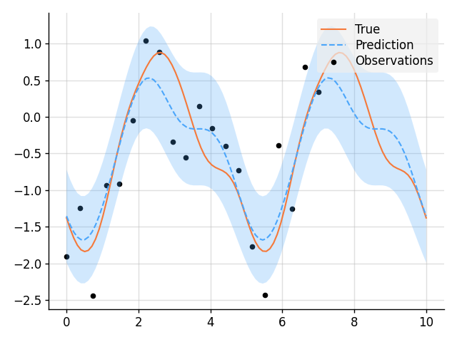
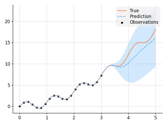
import matplotlib.pyplot as pltfrom wbml.plot import tweakfrom stheno import B, GP, EQ# Define points to predict at.x = B.linspace(0, 10, 100)x_obs = B.linspace(0, 7, 20)# Construct a prior.f = GP(EQ().periodic(5.0))# Sample a true, underlying function and noisy observations.f_true, y_obs = f.measure.sample(f(x), f(x_obs, 0.5))# Now condition on the observations to make predictions.f_post = f | (f(x_obs, 0.5), y_obs)mean, lower, upper = f_post(x).marginal_credible_bounds()# Plot result.plt.plot(x, f_true, label="True", style="test")plt.scatter(x_obs, y_obs, label="Observations", style="train", s=20)plt.plot(x, mean, label="Prediction", style="pred")plt.fill_between(x, lower, upper, style="pred")tweak()plt.savefig("readme_example1_simple_regression.png")plt.show()
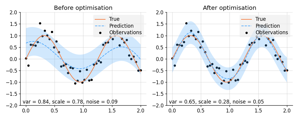
import lab as Bimport matplotlib.pyplot as pltimport torchfrom varz import Vars, minimise_l_bfgs_b, parametrised, Positivefrom wbml.plot import tweakfrom stheno.torch import EQ, GP# Increase regularisation because PyTorch defaults to 32-bit floats.B.epsilon = 1e-6# Define points to predict at.x = torch.linspace(0, 2, 100)x_obs = torch.linspace(0, 2, 50)# Sample a true, underlying function and observations with observation noise `0.05`.f_true = torch.sin(5 * x)y_obs = torch.sin(5 * x_obs) + 0.05**0.5 * torch.randn(50)def model(vs):"""Construct a model with learnable parameters."""p = vs.struct # Varz handles positivity (and other) constraints.kernel = p.variance.positive() * EQ().stretch(p.scale.positive())return GP(kernel), p.noise.positive()@parametriseddef model_alternative(vs, scale: Positive, variance: Positive, noise: Positive):"""Equivalent to :func:`model`, but with `@parametrised`."""kernel = variance * EQ().stretch(scale)return GP(kernel), noisevs = Vars(torch.float32)f, noise = model(vs)# Condition on observations and make predictions before optimisation.f_post = f | (f(x_obs, noise), y_obs)prior_before = f, noisepred_before = f_post(x, noise).marginal_credible_bounds()def objective(vs):f, noise = model(vs)evidence = f(x_obs, noise).logpdf(y_obs)return -evidence# Learn hyperparameters.minimise_l_bfgs_b(objective, vs)f, noise = model(vs)# Condition on observations and make predictions after optimisation.f_post = f | (f(x_obs, noise), y_obs)prior_after = f, noisepred_after = f_post(x, noise).marginal_credible_bounds()def plot_prediction(prior, pred):f, noise = priormean, lower, upper = predplt.scatter(x_obs, y_obs, label="Observations", style="train", s=20)plt.plot(x, f_true, label="True", style="test")plt.plot(x, mean, label="Prediction", style="pred")plt.fill_between(x, lower, upper, style="pred")plt.ylim(-2, 2)plt.text(0.02,0.02,f"var = {f.kernel.factor(0):.2f}, "f"scale = {f.kernel.factor(1).stretches[0]:.2f}, "f"noise = {noise:.2f}",transform=plt.gca().transAxes,)tweak()# Plot result.plt.figure(figsize=(10, 4))plt.subplot(1, 2, 1)plt.title("Before optimisation")plot_prediction(prior_before, pred_before)plt.subplot(1, 2, 2)plt.title("After optimisation")plot_prediction(prior_after, pred_after)plt.savefig("readme_example12_optimisation_varz.png")plt.show()
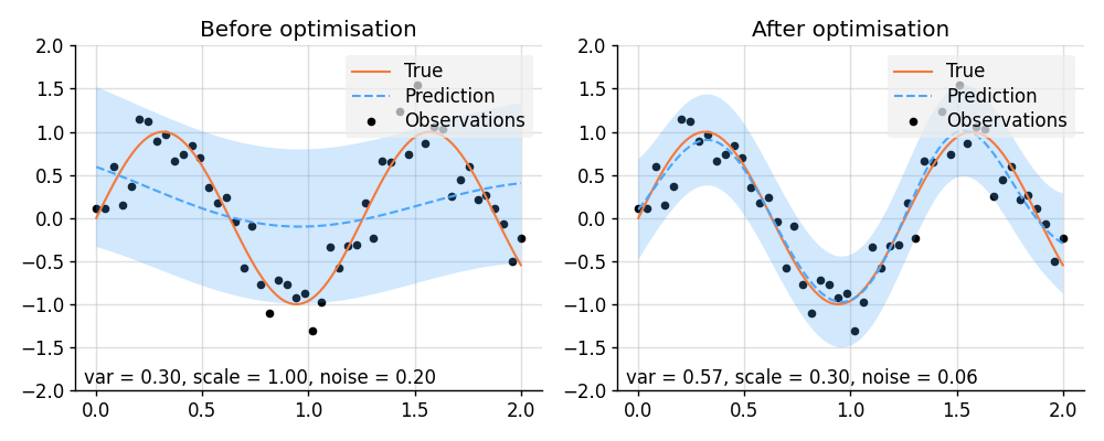
import lab as Bimport matplotlib.pyplot as pltimport torchfrom wbml.plot import tweakfrom stheno.torch import EQ, GP# Increase regularisation because PyTorch defaults to 32-bit floats.B.epsilon = 1e-6# Define points to predict at.x = torch.linspace(0, 2, 100)x_obs = torch.linspace(0, 2, 50)# Sample a true, underlying function and observations with observation noise `0.05`.f_true = torch.sin(5 * x)y_obs = torch.sin(5 * x_obs) + 0.05**0.5 * torch.randn(50)class Model(torch.nn.Module):"""A GP model with learnable parameters."""def __init__(self, init_var=0.3, init_scale=1, init_noise=0.2):super().__init__()# Ensure that the parameters are positive and make them learnable.self.log_var = torch.nn.Parameter(torch.log(torch.tensor(init_var)))self.log_scale = torch.nn.Parameter(torch.log(torch.tensor(init_scale)))self.log_noise = torch.nn.Parameter(torch.log(torch.tensor(init_noise)))def construct(self):self.var = torch.exp(self.log_var)self.scale = torch.exp(self.log_scale)self.noise = torch.exp(self.log_noise)kernel = self.var * EQ().stretch(self.scale)return GP(kernel), self.noisemodel = Model()f, noise = model.construct()# Condition on observations and make predictions before optimisation.f_post = f | (f(x_obs, noise), y_obs)prior_before = f, noisepred_before = f_post(x, noise).marginal_credible_bounds()# Perform optimisation.opt = torch.optim.Adam(model.parameters(), lr=5e-2)for _ in range(1000):opt.zero_grad()f, noise = model.construct()loss = -f(x_obs, noise).logpdf(y_obs)loss.backward()opt.step()f, noise = model.construct()# Condition on observations and make predictions after optimisation.f_post = f | (f(x_obs, noise), y_obs)prior_after = f, noisepred_after = f_post(x, noise).marginal_credible_bounds()def plot_prediction(prior, pred):f, noise = priormean, lower, upper = predplt.scatter(x_obs, y_obs, label="Observations", style="train", s=20)plt.plot(x, f_true, label="True", style="test")plt.plot(x, mean, label="Prediction", style="pred")plt.fill_between(x, lower, upper, style="pred")plt.ylim(-2, 2)plt.text(0.02,0.02,f"var = {f.kernel.factor(0):.2f}, "f"scale = {f.kernel.factor(1).stretches[0]:.2f}, "f"noise = {noise:.2f}",transform=plt.gca().transAxes,)tweak()# Plot result.plt.figure(figsize=(10, 4))plt.subplot(1, 2, 1)plt.title("Before optimisation")plot_prediction(prior_before, pred_before)plt.subplot(1, 2, 2)plt.title("After optimisation")plot_prediction(prior_after, pred_after)plt.savefig("readme_example13_optimisation_torch.png")plt.show()
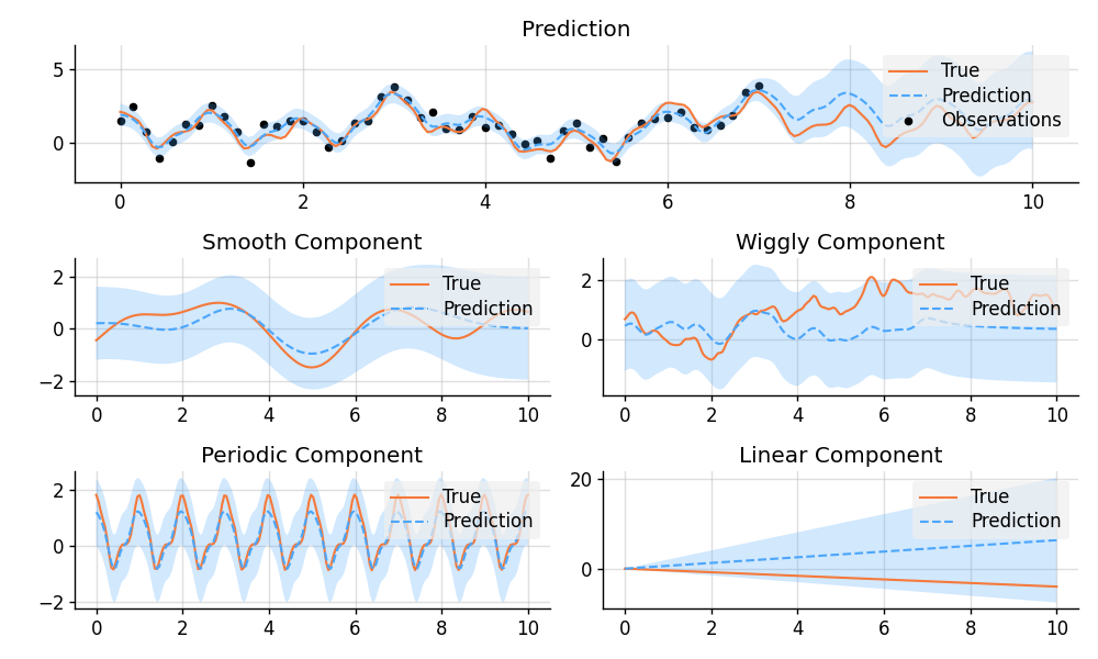
import matplotlib.pyplot as pltfrom wbml.plot import tweakfrom stheno import Measure, GP, EQ, RQ, Linear, Delta, Exp, BB.epsilon = 1e-10# Define points to predict at.x = B.linspace(0, 10, 200)x_obs = B.linspace(0, 7, 50)with Measure() as prior:# Construct a latent function consisting of four different components.f_smooth = GP(EQ())f_wiggly = GP(RQ(1e-1).stretch(0.5))f_periodic = GP(EQ().periodic(1.0))f_linear = GP(Linear())f = f_smooth + f_wiggly + f_periodic + 0.2 * f_linear# Let the observation noise consist of a bit of exponential noise.e_indep = GP(Delta())e_exp = GP(Exp())e = e_indep + 0.3 * e_exp# Sum the latent function and observation noise to get a model for the observations.y = f + 0.5 * e# Sample a true, underlying function and observations.(f_true_smooth,f_true_wiggly,f_true_periodic,f_true_linear,f_true,y_obs,) = prior.sample(f_smooth(x), f_wiggly(x), f_periodic(x), f_linear(x), f(x), y(x_obs))# Now condition on the observations and make predictions for the latent function and# its various components.post = prior | (y(x_obs), y_obs)pred_smooth = post(f_smooth(x))pred_wiggly = post(f_wiggly(x))pred_periodic = post(f_periodic(x))pred_linear = post(f_linear(x))pred_f = post(f(x))# Plot results.def plot_prediction(x, f, pred, x_obs=None, y_obs=None):plt.plot(x, f, label="True", style="test")if x_obs is not None:plt.scatter(x_obs, y_obs, label="Observations", style="train", s=20)mean, lower, upper = pred.marginal_credible_bounds()plt.plot(x, mean, label="Prediction", style="pred")plt.fill_between(x, lower, upper, style="pred")tweak()plt.figure(figsize=(10, 6))plt.subplot(3, 1, 1)plt.title("Prediction")plot_prediction(x, f_true, pred_f, x_obs, y_obs)plt.subplot(3, 2, 3)plt.title("Smooth Component")plot_prediction(x, f_true_smooth, pred_smooth)plt.subplot(3, 2, 4)plt.title("Wiggly Component")plot_prediction(x, f_true_wiggly, pred_wiggly)plt.subplot(3, 2, 5)plt.title("Periodic Component")plot_prediction(x, f_true_periodic, pred_periodic)plt.subplot(3, 2, 6)plt.title("Linear Component")plot_prediction(x, f_true_linear, pred_linear)plt.savefig("readme_example2_decomposition.png")plt.show()
import matplotlib.pyplot as pltimport tensorflow as tfimport wbml.out as outfrom varz.spec import parametrised, Positivefrom varz.tensorflow import Vars, minimise_l_bfgs_bfrom wbml.plot import tweakfrom stheno.tensorflow import B, Measure, GP, EQ, Delta# Define points to predict at.x = B.linspace(tf.float64, 0, 5, 100)x_obs = B.linspace(tf.float64, 0, 3, 20)@parametriseddef model(vs,u_var: Positive = 0.5,u_scale: Positive = 0.5,noise: Positive = 0.5,alpha: Positive = 1.2,):with Measure():# Random fluctuation:u = GP(u_var * EQ().stretch(u_scale))# Construct model.f = u + (lambda x: x**alpha)return f, noise# Sample a true, underlying function and observations.vs = Vars(tf.float64)f_true = x**1.8 + B.sin(2 * B.pi * x)f, y = model(vs)post = f.measure | (f(x), f_true)y_obs = post(f(x_obs)).sample()def objective(vs):f, noise = model(vs)evidence = f(x_obs, noise).logpdf(y_obs)return -evidence# Learn hyperparameters.minimise_l_bfgs_b(objective, vs, jit=True)f, noise = model(vs)# Print the learned parameters.out.kv("Prior", f.display(out.format))vs.print()# Condition on the observations to make predictions.f_post = f | (f(x_obs, noise), y_obs)mean, lower, upper = f_post(x).marginal_credible_bounds()# Plot result.plt.plot(x, B.squeeze(f_true), label="True", style="test")plt.scatter(x_obs, B.squeeze(y_obs), label="Observations", style="train", s=20)plt.plot(x, mean, label="Prediction", style="pred")plt.fill_between(x, lower, upper, style="pred")tweak()plt.savefig("readme_example3_parametric.png")plt.show()
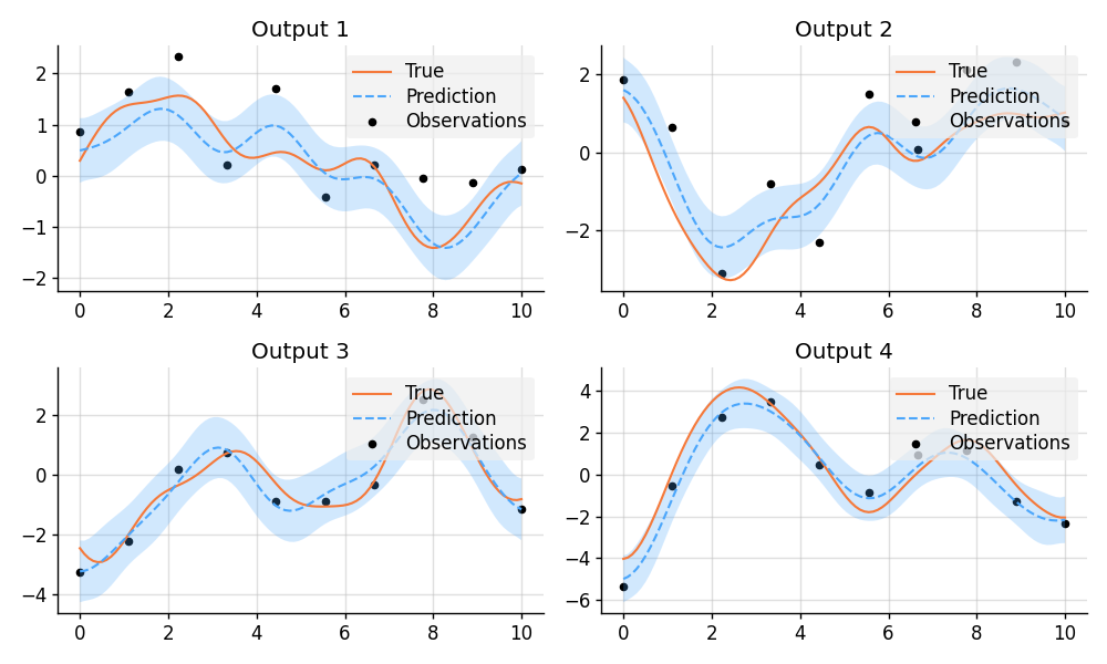
import matplotlib.pyplot as pltfrom wbml.plot import tweakfrom stheno import B, Measure, GP, EQ, Deltaclass VGP:"""A vector-valued GP."""def __init__(self, ps):self.ps = psdef __add__(self, other):return VGP([f + g for f, g in zip(self.ps, other.ps)])def lmatmul(self, A):m, n = A.shapeps = [0 for _ in range(m)]for i in range(m):for j in range(n):ps[i] += A[i, j] * self.ps[j]return VGP(ps)# Define points to predict at.x = B.linspace(0, 10, 100)x_obs = B.linspace(0, 10, 10)# Model parameters:m = 2p = 4H = B.randn(p, m)with Measure() as prior:# Construct latent functions.us = VGP([GP(EQ()) for _ in range(m)])# Construct multi-output prior.fs = us.lmatmul(H)# Construct noise.e = VGP([GP(0.5 * Delta()) for _ in range(p)])# Construct observation model.ys = e + fs# Sample a true, underlying function and observations.samples = prior.sample(*(p(x) for p in fs.ps), *(p(x_obs) for p in ys.ps))fs_true, ys_obs = samples[:p], samples[p:]# Compute the posterior and make predictions.post = prior.condition(*((p(x_obs), y_obs) for p, y_obs in zip(ys.ps, ys_obs)))preds = [post(p(x)) for p in fs.ps]# Plot results.def plot_prediction(x, f, pred, x_obs=None, y_obs=None):plt.plot(x, f, label="True", style="test")if x_obs is not None:plt.scatter(x_obs, y_obs, label="Observations", style="train", s=20)mean, lower, upper = pred.marginal_credible_bounds()plt.plot(x, mean, label="Prediction", style="pred")plt.fill_between(x, lower, upper, style="pred")tweak()plt.figure(figsize=(10, 6))for i in range(4):plt.subplot(2, 2, i + 1)plt.title(f"Output {i + 1}")plot_prediction(x, fs_true[i], preds[i], x_obs, ys_obs[i])plt.savefig("readme_example4_multi-output.png")plt.show()
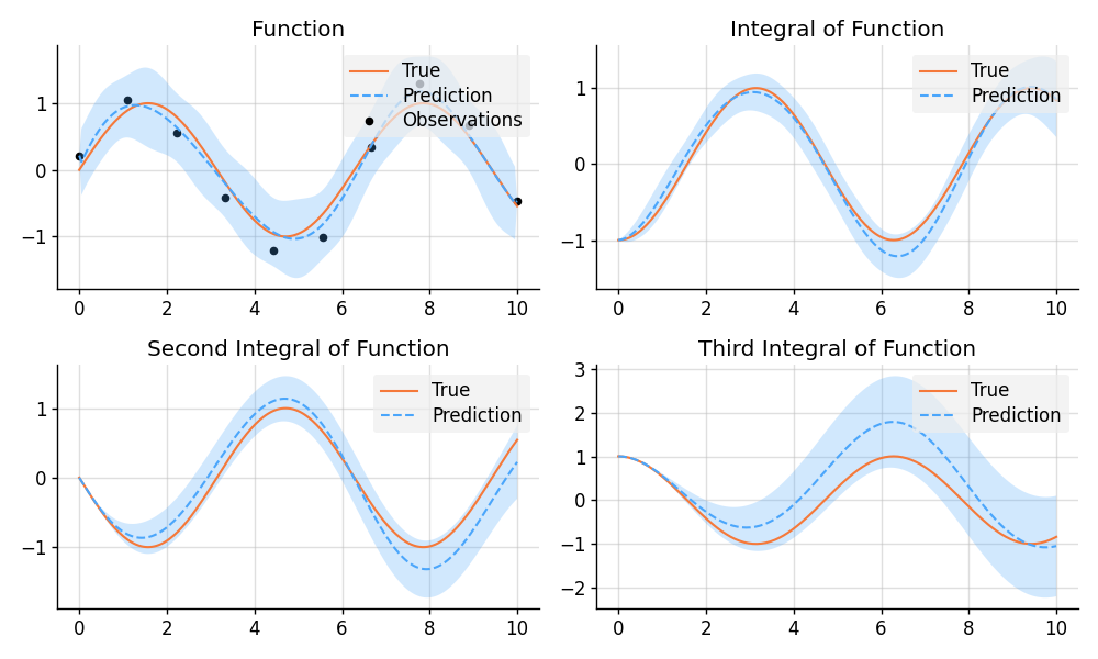
import matplotlib.pyplot as pltimport numpy as npimport tensorflow as tfimport wbml.plotfrom stheno.tensorflow import B, Measure, GP, EQ, Delta# Define points to predict at.x = B.linspace(tf.float64, 0, 10, 200)x_obs = B.linspace(tf.float64, 0, 10, 10)with Measure() as prior:# Construct a model.f = 0.7 * GP(EQ()).stretch(1.5)e = 0.2 * GP(Delta())# Construct derivatives.df = f.diff()ddf = df.diff()dddf = ddf.diff() + e# Fix the integration constants.zero = B.cast(tf.float64, 0)one = B.cast(tf.float64, 1)prior = prior | ((f(zero), one), (df(zero), zero), (ddf(zero), -one))# Sample observations.y_obs = B.sin(x_obs) + 0.2 * B.randn(*x_obs.shape)# Condition on the observations to make predictions.post = prior | (dddf(x_obs), y_obs)# And make predictions.pred_iiif = post(f)(x)pred_iif = post(df)(x)pred_if = post(ddf)(x)pred_f = post(dddf)(x)# Plot result.def plot_prediction(x, f, pred, x_obs=None, y_obs=None):plt.plot(x, f, label="True", style="test")if x_obs is not None:plt.scatter(x_obs, y_obs, label="Observations", style="train", s=20)mean, lower, upper = pred.marginal_credible_bounds()plt.plot(x, mean, label="Prediction", style="pred")plt.fill_between(x, lower, upper, style="pred")wbml.plot.tweak()plt.figure(figsize=(10, 6))plt.subplot(2, 2, 1)plt.title("Function")plot_prediction(x, np.sin(x), pred_f, x_obs=x_obs, y_obs=y_obs)plt.subplot(2, 2, 2)plt.title("Integral of Function")plot_prediction(x, -np.cos(x), pred_if)plt.subplot(2, 2, 3)plt.title("Second Integral of Function")plot_prediction(x, -np.sin(x), pred_iif)plt.subplot(2, 2, 4)plt.title("Third Integral of Function")plot_prediction(x, np.cos(x), pred_iiif)plt.savefig("readme_example5_integration.png")plt.show()
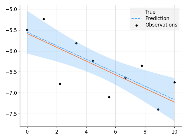
import matplotlib.pyplot as pltimport wbml.out as outfrom wbml.plot import tweakfrom stheno import B, Measure, GPB.epsilon = 1e-10 # Very slightly regularise.# Define points to predict at.x = B.linspace(0, 10, 200)x_obs = B.linspace(0, 10, 10)with Measure() as prior:# Construct a linear model.slope = GP(1)intercept = GP(5)f = slope * (lambda x: x) + intercept# Sample a slope, intercept, underlying function, and observations.true_slope, true_intercept, f_true, y_obs = prior.sample(slope(0), intercept(0), f(x), f(x_obs, 0.2))# Condition on the observations to make predictions.post = prior | (f(x_obs, 0.2), y_obs)mean, lower, upper = post(f(x)).marginal_credible_bounds()out.kv("True slope", true_slope[0, 0])out.kv("Predicted slope", post(slope(0)).mean[0, 0])out.kv("True intercept", true_intercept[0, 0])out.kv("Predicted intercept", post(intercept(0)).mean[0, 0])# Plot result.plt.plot(x, f_true, label="True", style="test")plt.scatter(x_obs, y_obs, label="Observations", style="train", s=20)plt.plot(x, mean, label="Prediction", style="pred")plt.fill_between(x, lower, upper, style="pred")tweak()plt.savefig("readme_example6_blr.png")plt.show()
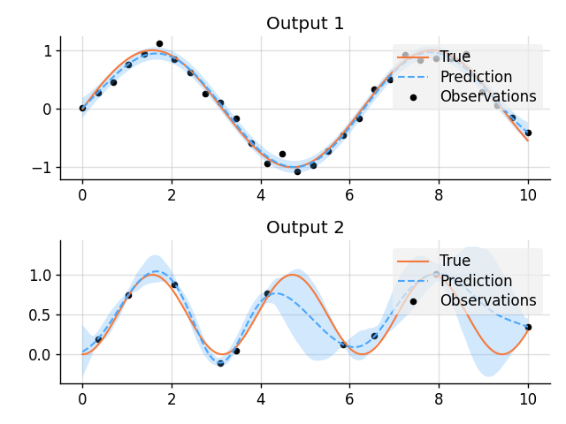
import matplotlib.pyplot as pltimport numpy as npimport tensorflow as tffrom varz.spec import parametrised, Positivefrom varz.tensorflow import Vars, minimise_l_bfgs_bfrom wbml.plot import tweakfrom stheno.tensorflow import B, GP, EQ# Define points to predict at.x = B.linspace(tf.float64, 0, 10, 200)x_obs1 = B.linspace(tf.float64, 0, 10, 30)inds2 = np.random.permutation(len(x_obs1))[:10]x_obs2 = B.take(x_obs1, inds2)# Construction functions to predict and observations.f1_true = B.sin(x)f2_true = B.sin(x) ** 2y1_obs = B.sin(x_obs1) + 0.1 * B.randn(*x_obs1.shape)y2_obs = B.sin(x_obs2) ** 2 + 0.1 * B.randn(*x_obs2.shape)@parametriseddef model(vs,var1: Positive = 1,scale1: Positive = 1,noise1: Positive = 0.1,var2: Positive = 1,scale2: Positive = 1,noise2: Positive = 0.1,):# Build layers:f1 = GP(var1 * EQ().stretch(scale1))f2 = GP(var2 * EQ().stretch(scale2))return (f1, noise1), (f2, noise2)def objective(vs):(f1, noise1), (f2, noise2) = model(vs)x1 = x_obs1x2 = B.stack(x_obs2, B.take(y1_obs, inds2), axis=1)evidence = f1(x1, noise1).logpdf(y1_obs) + f2(x2, noise2).logpdf(y2_obs)return -evidence# Learn hyperparameters.vs = Vars(tf.float64)minimise_l_bfgs_b(objective, vs)# Compute posteriors.(f1, noise1), (f2, noise2) = model(vs)x1 = x_obs1x2 = B.stack(x_obs2, B.take(y1_obs, inds2), axis=1)f1_post = f1 | (f1(x1, noise1), y1_obs)f2_post = f2 | (f2(x2, noise2), y2_obs)# Predict first output.mean1, lower1, upper1 = f1_post(x).marginal_credible_bounds()# Predict second output with Monte Carlo.samples = [f2_post(B.stack(x, f1_post(x).sample()[:, 0], axis=1)).sample()[:, 0]for _ in range(100)]mean2 = np.mean(samples, axis=0)lower2 = np.percentile(samples, 2.5, axis=0)upper2 = np.percentile(samples, 100 - 2.5, axis=0)# Plot result.plt.figure()plt.subplot(2, 1, 1)plt.title("Output 1")plt.plot(x, f1_true, label="True", style="test")plt.scatter(x_obs1, y1_obs, label="Observations", style="train", s=20)plt.plot(x, mean1, label="Prediction", style="pred")plt.fill_between(x, lower1, upper1, style="pred")tweak()plt.subplot(2, 1, 2)plt.title("Output 2")plt.plot(x, f2_true, label="True", style="test")plt.scatter(x_obs2, y2_obs, label="Observations", style="train", s=20)plt.plot(x, mean2, label="Prediction", style="pred")plt.fill_between(x, lower2, upper2, style="pred")tweak()plt.savefig("readme_example7_gpar.png")plt.show()
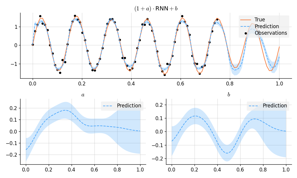
import matplotlib.pyplot as pltimport numpy as npimport tensorflow as tffrom varz.spec import parametrised, Positivefrom varz.tensorflow import Vars, minimise_adamfrom wbml.net import rnn as rnn_constructorfrom wbml.plot import tweakfrom stheno.tensorflow import B, Measure, GP, EQ# Increase regularisation because we are dealing with `tf.float32`s.B.epsilon = 1e-6# Construct points which to predict at.x = B.linspace(tf.float32, 0, 1, 100)[:, None]inds_obs = B.range(0, int(0.75 * len(x))) # Train on the first 75% only.x_obs = B.take(x, inds_obs)# Construct function and observations.# Draw random modulation functions.a_true = GP(1e-2 * EQ().stretch(0.1))(x).sample()b_true = GP(1e-2 * EQ().stretch(0.1))(x).sample()# Construct the true, underlying function.f_true = (1 + a_true) * B.sin(2 * np.pi * 7 * x) + b_true# Add noise.y_true = f_true + 0.1 * B.randn(*f_true.shape)# Normalise and split.f_true = (f_true - B.mean(y_true)) / B.std(y_true)y_true = (y_true - B.mean(y_true)) / B.std(y_true)y_obs = B.take(y_true, inds_obs)@parametriseddef model(vs, a_scale: Positive = 0.1, b_scale: Positive = 0.1, noise: Positive = 0.01):# Construct an RNN.f_rnn = rnn_constructor(output_size=1, widths=(10,), nonlinearity=B.tanh, final_dense=True)# Set the weights for the RNN.num_weights = f_rnn.num_weights(input_size=1)weights = Vars(tf.float32, source=vs.get(shape=(num_weights,), name="rnn"))f_rnn.initialise(input_size=1, vs=weights)with Measure():# Construct GPs that modulate the RNN.a = GP(1e-2 * EQ().stretch(a_scale))b = GP(1e-2 * EQ().stretch(b_scale))# GP-RNN model:f_gp_rnn = (1 + a) * (lambda x: f_rnn(x)) + breturn f_rnn, f_gp_rnn, noise, a, bdef objective_rnn(vs):f_rnn, _, _, _, _ = model(vs)return B.mean((f_rnn(x_obs) - y_obs) ** 2)def objective_gp_rnn(vs):_, f_gp_rnn, noise, _, _ = model(vs)evidence = f_gp_rnn(x_obs, noise).logpdf(y_obs)return -evidence# Pretrain the RNN.vs = Vars(tf.float32)minimise_adam(objective_rnn, vs, rate=5e-3, iters=1000, trace=True, jit=True)# Jointly train the RNN and GPs.minimise_adam(objective_gp_rnn, vs, rate=1e-3, iters=1000, trace=True, jit=True)_, f_gp_rnn, noise, a, b = model(vs)# Condition.post = f_gp_rnn.measure | (f_gp_rnn(x_obs, noise), y_obs)# Predict and plot results.plt.figure(figsize=(10, 6))plt.subplot(2, 1, 1)plt.title("$(1 + a)\\cdot {}$RNN${} + b$")plt.plot(x, f_true, label="True", style="test")plt.scatter(x_obs, y_obs, label="Observations", style="train", s=20)mean, lower, upper = post(f_gp_rnn(x)).marginal_credible_bounds()plt.plot(x, mean, label="Prediction", style="pred")plt.fill_between(x, lower, upper, style="pred")tweak()plt.subplot(2, 2, 3)plt.title("$a$")mean, lower, upper = post(a(x)).marginal_credible_bounds()plt.plot(x, mean, label="Prediction", style="pred")plt.fill_between(x, lower, upper, style="pred")tweak()plt.subplot(2, 2, 4)plt.title("$b$")mean, lower, upper = post(b(x)).marginal_credible_bounds()plt.plot(x, mean, label="Prediction", style="pred")plt.fill_between(x, lower, upper, style="pred")tweak()plt.savefig(f"readme_example8_gp-rnn.png")plt.show()
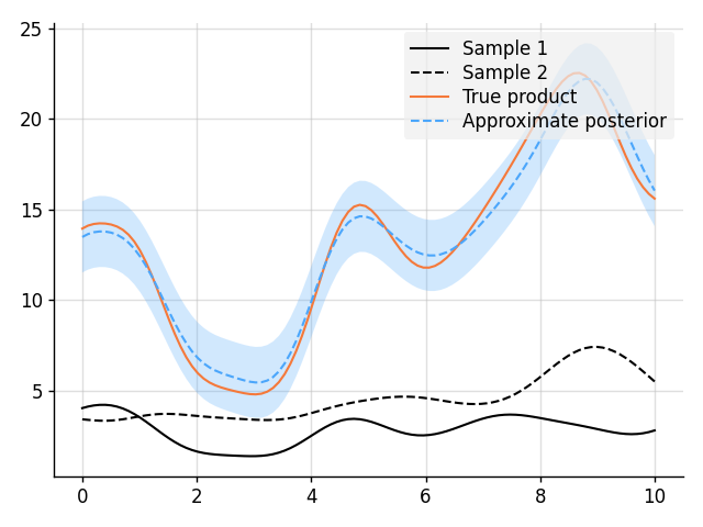
import matplotlib.pyplot as pltfrom wbml.plot import tweakfrom stheno import B, Measure, GP, EQ# Define points to predict at.x = B.linspace(0, 10, 100)with Measure() as prior:f1 = GP(3, EQ())f2 = GP(3, EQ())# Compute the approximate product.f_prod = f1 * f2# Sample two functions.s1, s2 = prior.sample(f1(x), f2(x))# Predict.f_prod_post = f_prod | ((f1(x), s1), (f2(x), s2))mean, lower, upper = f_prod_post(x).marginal_credible_bounds()# Plot result.plt.plot(x, s1, label="Sample 1", style="train")plt.plot(x, s2, label="Sample 2", style="train", ls="--")plt.plot(x, s1 * s2, label="True product", style="test")plt.plot(x, mean, label="Approximate posterior", style="pred")plt.fill_between(x, lower, upper, style="pred")tweak()plt.savefig("readme_example9_product.png")plt.show()
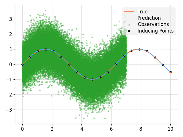
import matplotlib.pyplot as pltimport wbml.out as outfrom wbml.plot import tweakfrom stheno import B, GP, EQ, PseudoObs# Define points to predict at.x = B.linspace(0, 10, 100)x_obs = B.linspace(0, 7, 50_000)x_ind = B.linspace(0, 10, 20)# Construct a prior.f = GP(EQ().periodic(2 * B.pi))# Sample a true, underlying function and observations.f_true = B.sin(x)y_obs = B.sin(x_obs) + B.sqrt(0.5) * B.randn(*x_obs.shape)# Compute a pseudo-point approximation of the posterior.obs = PseudoObs(f(x_ind), (f(x_obs, 0.5), y_obs))# Compute the ELBO.out.kv("ELBO", obs.elbo(f.measure))# Compute the approximate posterior.f_post = f | obs# Make predictions with the approximate posterior.mean, lower, upper = f_post(x).marginal_credible_bounds()# Plot result.plt.plot(x, f_true, label="True", style="test")plt.scatter(x_obs,y_obs,label="Observations",style="train",c="tab:green",alpha=0.35,)plt.scatter(x_ind,obs.mu(f.measure)[:, 0],label="Inducing Points",style="train",s=20,)plt.plot(x, mean, label="Prediction", style="pred")plt.fill_between(x, lower, upper, style="pred")tweak()plt.savefig("readme_example10_sparse.png")plt.show()
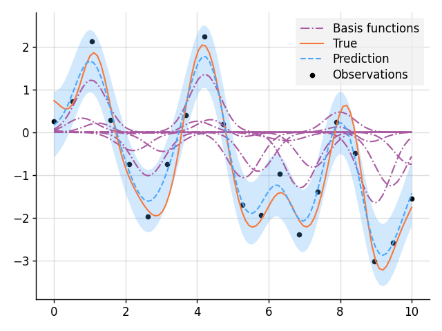
import matplotlib.pyplot as pltfrom wbml.plot import tweakfrom stheno import B, Measure, GP, EQ# Define points to predict at.x = B.linspace(0, 10, 100)x_obs = B.linspace(0, 10, 20)with Measure() as prior:w = lambda x: B.exp(-(x**2) / 0.5) # Basis functionb = [(w * GP(EQ())).shift(xi) for xi in x_obs] # Weighted basis functionsf = sum(b)# Sample a true, underlying function and observations.f_true, y_obs = prior.sample(f(x), f(x_obs, 0.2))# Condition on the observations to make predictions.post = prior | (f(x_obs, 0.2), y_obs)# Plot result.for i, bi in enumerate(b):mean, lower, upper = post(bi(x)).marginal_credible_bounds()kw_args = {"label": "Basis functions"} if i == 0 else {}plt.plot(x, mean, style="pred2", **kw_args)plt.plot(x, f_true, label="True", style="test")plt.scatter(x_obs, y_obs, label="Observations", style="train", s=20)mean, lower, upper = post(f(x)).marginal_credible_bounds()plt.plot(x, mean, label="Prediction", style="pred")plt.fill_between(x, lower, upper, style="pred")tweak()plt.savefig("readme_example11_nonparametric_basis.png")plt.show()